Pharmacokinetics & Dosing Concepts
Effective Half-Life
The effective half-life is the single half-life that reproduces a drug's observed accumulation on repeated dosing, replacing a terminal value that may describe a negligible part of exposure.
For a drug whose concentration falls along several exponential phases, no single half-life describes it, and the terminal one describes only the last phase. The effective half-life answers a more useful question: what half-life would a simple one-phase drug need in order to accumulate exactly as much as this one does on the same schedule? It is calculated backwards from the observed accumulation ratio and the dosing interval, and because it is anchored to what repeated dosing actually did, it predicts time to plateau and washout better than a slope fitted to the tail.
The gap between the two numbers can be large. A compound that distributes into a deep tissue compartment and returns from it slowly shows a long terminal phase at concentrations well under anything active, while the exposure that matters turns over in a fraction of that time. Depot products invert the problem: their apparent decline reflects the formulation emptying, so the number describes the polymer rather than the peptide. Regulatory guidance on multiple-dose pharmacokinetics accordingly asks for accumulation data rather than a terminal slope alone when justifying a dosing interval.
Using the effective value changes practical conclusions in both directions. It shortens the expected time to steady state for drugs with a long shallow tail, and it lengthens the expected washout for drugs whose slow release keeps concentrations up.
The reason this matters commercially is that a terminal half-life is the easiest number to inflate. Sample longer, use a more sensitive assay, and the fitted terminal slope flattens while nothing about the compound has changed. Product literature quoting the largest half-life anyone has published, with no accumulation data behind it, is describing assay sensitivity. The honest test is whether the observed plateau matches what that half-life predicts.
Worked examples — first-order elimination
Each curve solves C(t) = C₀·e^(−kt) with k = ln2 ÷ t½. The dots mark successive half-lives, which is why the same fraction disappears in every interval regardless of where you start.
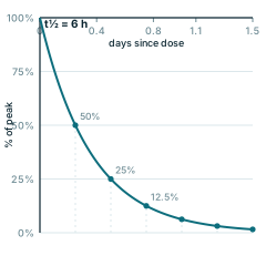
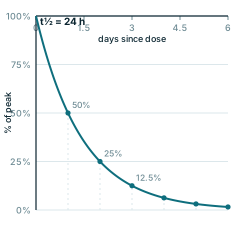
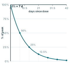
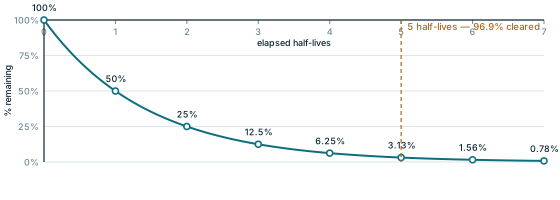
Every panel is redrawn from its own equation by scripts/glossary-figures.js — no traced or stock artwork, and a rebuild is byte-identical.