Pharmacokinetics & Dosing Concepts
Dosing Interval
The dosing interval is the time between successive doses, and its ratio to the half-life determines how far concentrations swing and how much drug accumulates.
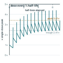
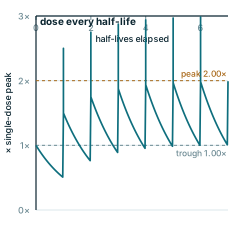
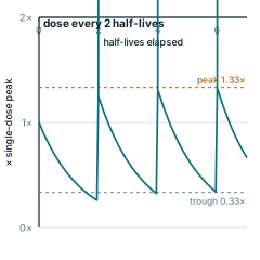
The interval between doses is one of the two variables under a prescriber's control. Its consequences follow from a single comparison: how long the interval is in units of half-life. For a drug declining exponentially, concentration falls by a factor of two raised to the power of that ratio between one peak and the next trough, so an interval of one half-life gives a twofold swing and an interval of four half-lives a sixteen-fold one. Short intervals give flat profiles with substantial accumulation; long ones give spiky profiles with almost none.
The incretin analogues were designed to move along this axis. Native glucagon-like peptide-1 survives about two minutes and is usable only as an infusion. Liraglutide, at roughly thirteen hours, is a daily injection. Semaglutide at about a week and tirzepatide at around five days are weekly. Elsewhere the interval is itself the active variable: gonadotropin-releasing hormone must be delivered in pulses roughly every ninety minutes to sustain gonadotropin secretion, because continuous exposure to the same molecule downregulates the receptor and suppresses the axis.
Choosing an interval is a negotiation between the therapeutic window and adherence. A wide window tolerates intervals well beyond the half-life, trading fluctuation for convenience. A narrow one forces intervals at or below the half-life, because the peak has to stay below toxicity while the trough stays above efficacy.
The frequent mistake is assuming that splitting the same total amount into more frequent doses is always an improvement. For receptor systems that decode frequency, more frequent is a different signal, not a smoother one, and the pulsatile axes are where that misjudgement causes the most trouble. Intervals taken from rodent studies are worse still, since rodent clearance is generally much faster and the schedule does not translate.
Worked examples — accumulation to steady state
Repeat doses are summed by superposition: every dose still in the body keeps decaying while the next one lands. Peak and trough have closed forms — 1/(1−e^(−kτ)) and that value times e^(−kτ) — so the plateau height is set entirely by the dosing interval relative to the half-life.
Every panel is redrawn from its own equation by scripts/glossary-figures.js — no traced or stock artwork, and a rebuild is byte-identical.